# Poor naming
x <- c(10, 20, 30, 40, 50)
y <- mean(x)

# Better naming
netball_scores <- c(10, 20, 30, 40, 50)
average_score <- mean(netball_scores)5 Coding Principles - Practical
5.1 Good Coding Principles
In the reading for this week, we covered some basic ideas relating to ‘good coding practices’.
There are a few things you can do in R to maintain readable, logical code, which we’ll cover below.
Use Descriptive Variable and Function Names
Using clear and descriptive names for variables and functions helps others (and your future self) understand what your code is doing without needing to dive into the details.
For example:
In this example, [netball_scores] and [average_score] clearly convey what the data represents.
Organise Code into Sections
Organising your R script into sections helps break down the code into logical parts, making it easier to follow.
You can use comments and separators (e.g., #, -, =, *) to create clear sections.
For example:
# ===============================
# 1. Loading Required Libraries
# ===============================
library(ggplot2)
library(dplyr)
Attaching package: 'dplyr'The following objects are masked from 'package:stats':
filter, lagThe following objects are masked from 'package:base':
intersect, setdiff, setequal, union# ===============================
# 2. Data Preparation
# ===============================
# Creating a synthetic dataset for demonstration
netball_data <- data.frame(
Player = c("Alice", "Bella", "Catherine", "Diana", "Emily"),
Position = c("Goal Shooter", "Wing Attack", "Goal Keeper", "Centre", "Goal Defense"),
Goals = c(45, 30, 0, 15, 5),
Assists = c(10, 25, 5, 20, 10)
)
# ===============================
# 3. Data Analysis
# ===============================
# Calculating the average goals scored
average_goals <- mean(netball_data$Goals)
# ===============================
# 4. Data Visualisation
# ===============================
# Plotting goals scored by each player
ggplot(netball_data, aes(x = Player, y = Goals)) +
geom_bar(stat = "identity") +
ggtitle("Goals Scored by Each Player")
Here, I’ve divided the script into four sections: loading libraries, data preparation, data analysis, and data visualisation. This structure helps you (and others) quickly locate parts of the script.
Commenting Your Code
Comments are essential for explaining why you wrote your code in a certain way. They should describe the purpose of complex code blocks, any assumptions made, and non-obvious decisions.
# Calculate the average goals scored by players
average_goals <- mean(netball_data$Goals)

# Plotting the goals scored by each player to identify top performers
ggplot(netball_data, aes(x = Player, y = Goals)) +
  geom_bar(stat = "identity") +
  ggtitle("Goals Scored by Each Player")
Notice that comments clarify the intention behind each operation, making it easier for someone else (or yourself in the future) to understand your code.
Consistent Indentation and Formatting
Consistent indentation and formatting improve readability. In R, it’s common to use two or four spaces for indentation. This helps differentiate between different code blocks.
For example:
# Poorly formatted code
average_goals<-mean(netball_data$Goals)

ggplot(netball_data,aes(x=Player,y=Goals))+geom_bar(stat="identity")+ggtitle("Goals Scored by Each Player")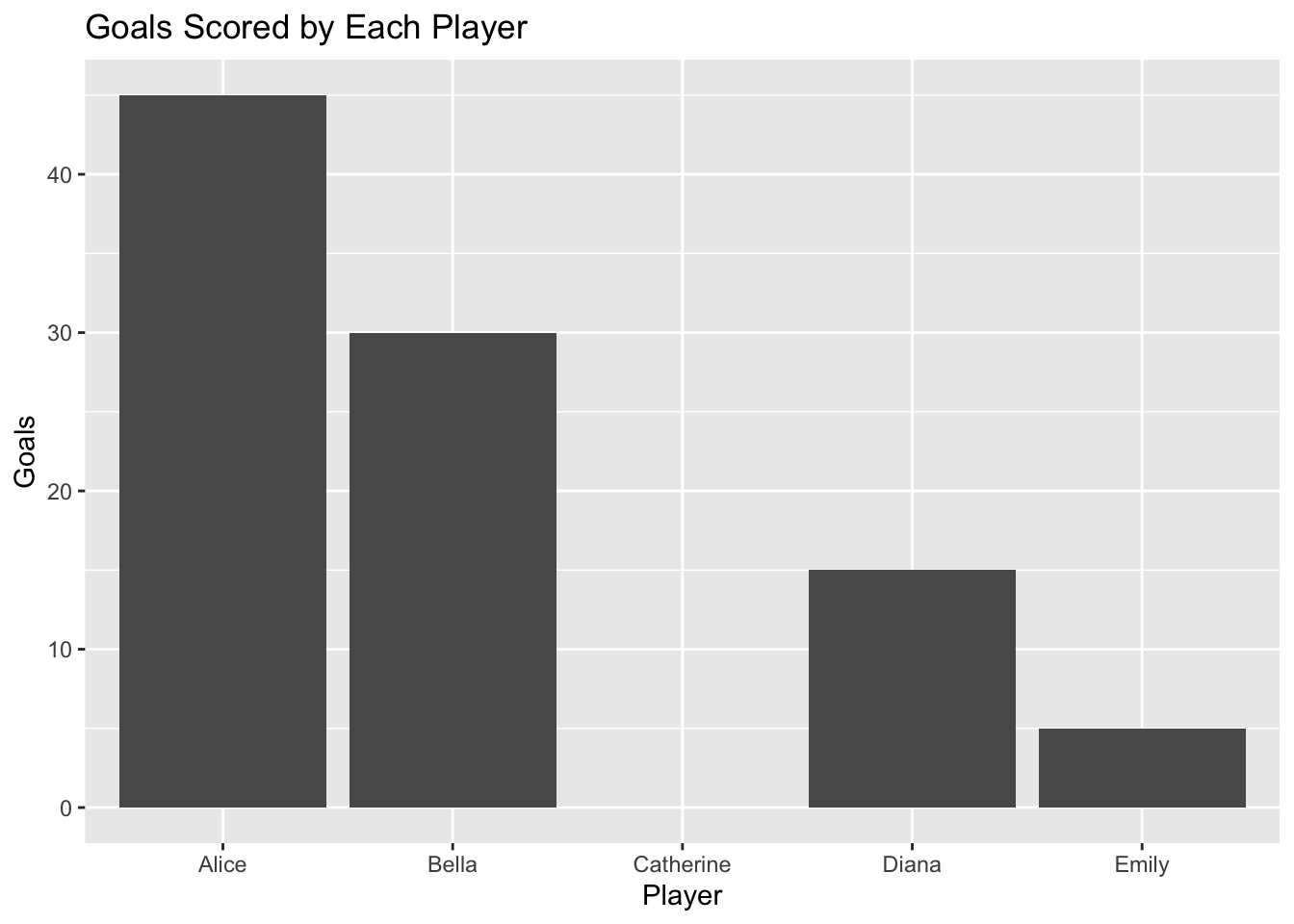
# Well-formatted code
average_goals <- mean(netball_data$Goals)

ggplot(netball_data, aes(x = Player, y = Goals)) +
  geom_bar(stat = "identity") +
  ggtitle("Goals Scored by Each Player")
Well-formatted code is much easier to read and debug.
Avoid Hard-Coding Values
Avoid hard-coding values directly in your code. Instead, use variables to store these values, which makes your code more flexible and easier to update.
For example:
# Hard-coded value
discounted_price <- 100 * 0.9

# Using a variable
original_price <- 100
discount_rate <- 0.9
discounted_price <- original_price * discount_rate
If the [discount_rate] changes, you only need to update it in one place.
Write Reusable Functions
Encapsulate repetitive tasks in functions. This not only makes your code cleaner but also makes it easier to reuse and maintain.
For example:
# Function to calculate average and plot results
analyse_performance <- function(data, score_column, title) {
  average_score <- mean(data[[score_column]])
  print(paste("Average Score:", average_score))

  ggplot(data, aes_string(x = "Player", y = score_column)) +
    geom_bar(stat = "identity") +
    ggtitle(title)
}

# Using the function
analyse_performance(netball_data, "Goals", "Goals Scored by Each Player")
[1] "Average Score: 19"Warning: `aes_string()` was deprecated in ggplot2 3.0.0.
ℹ Please use tidy evaluation idioms with `aes()`.
ℹ See also `vignette("ggplot2-in-packages")` for more information.
analyse_performance(netball_data, "Assists", "Assists by Each Player")[1] "Average Score: 14"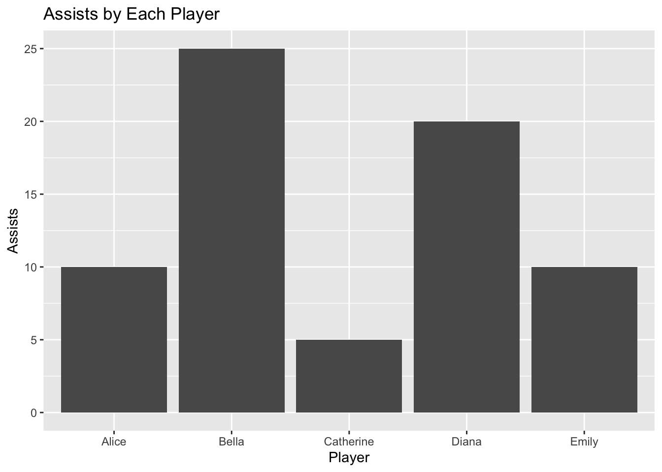
This function can be reused for different score columns, reducing code duplication and improving clarity.
5.2 Using Scripts
To conclude this section, we will work through a sequence of simple coding tasks in R. These will prepare the ground for next week, as well as give you an opportunity to ensure you fully understand how scripts in R and RStudio ‘work’.
Task 1: Writing a Simple Script
Task: Write a simple script that prints something to the console.
Show code
# Simple script
print("Hello, World!")
Task 2: Defining and Using Variables
Task: Create variables [a] = 5 and [b] = 3. Write a script that calculates the sum, difference, product, and quotient of these two variables and prints each result.
Example:
Show code
# Defining variables
a <- 5
b <- 3

# Performing calculations
sum_result <- a + b
difference_result <- a - b
product_result <- a * b
quotient_result <- a / b

# Printing results
print(paste("Sum:", sum_result))
print(paste("Difference:", difference_result))
print(paste("Product:", product_result))
print(paste("Quotient:", quotient_result))
Task 3: Using Functions
Task: Write a function square() that takes one argument and returns the square of that number.
Test it by squaring the number 4.
Show code
# Defining the function
square <- function(x) {
  return(x^2)
}

# Testing the function
result <- square(4)
print(result)
Task 4: Looping Through a Sequence
Task: Write a script that loops through the numbers 1 to 10 and prints each number multiplied by 2.
Show code
# Looping through numbers 1 to 10
for (i in 1:10) {
  print(i * 2)
}
Task 5: Conditional Statements
Task: Write a script that checks if a number is positive, negative, or zero.
Test it with the number 7.
Show code
# Defining the number
num <- 7

# Checking if the number is positive, negative, or zero
if (num > 0) {
  print("The number is positive.")
} else if (num < 0) {
  print("The number is negative.")
} else {
  print("The number is zero.")
}
Task 6: Using Data Frames
Task: Create a data frame with columns [Name] and [Age], then write a script that adds a new row to the data frame.
Show code
# Creating a data frame
df <- data.frame(Name = c("Alice", "Bob"), Age = c(25, 30))

# Adding a new row
new_row <- data.frame(Name = "Charlie", Age = 35)
df <- rbind(df, new_row)

# Printing the updated data frame
print(df)
Task 7: Reading and Writing Data to Files
Task: Write a script that writes a data frame to a CSV file and then reads the data back into R.
Show code
# Creating a data frame
df <- data.frame(Name = c("Alice", "Bob"), Age = c(25, 30))

# Writing the data frame to a CSV file
write.csv(df, "students.csv", row.names = FALSE)

# Reading the CSV file back into R
new_df <- read.csv("students.csv")

# Printing the read data
print(new_df)
Task 8: Plotting a Simple Graph
Task: Write a script that generates a simple scatter plot of two numeric vectors [x] and [y].
Show code
# Defining two numeric vectors
x <- c(1, 2, 3, 4, 5)
y <- c(2, 4, 6, 8, 10)

# Creating a scatter plot
plot(x, y, main = "Simple Scatter Plot", xlab = "X Values", ylab = "Y Values", col = "blue")
Task 9: Scripting with Libraries
Task: Load the ggplot2 library, then use it to create a bar plot of a simple data set.
Show code
# Loading ggplot2
library(ggplot2)

# Creating a simple data set
data <- data.frame(Category = c("A", "B", "C"), Values = c(3, 5, 8))

# Creating a bar plot
ggplot(data, aes(x = Category, y = Values)) +
  geom_bar(stat = "identity") +
  theme_minimal()
Task 10: Sourcing a Script
Task: Save one of the previous tasks as a script and demonstrate how to source and run it from another R script.
Show code
# Source the script using the name you gave it earlier"
source("Week Two Saved Script.R")